Mortgage Simulation

Background

This is a short explanation of the simulation implementation we did in the research Information problems in the mortgage market in Israel: price dispersion and search. For more information one can read the final report or dive even more into technical details published in the draft with the annexes. sadly, the report was published solely in Hebrew, though there is an extended abstract (8 pages long) in English at this link

The data-base used for the mortgage research consisted of nearly all mortgage data documented by the 3 largest banks in Israel in the years 2015-2017. In addition, we had all official mortgage bids consumers received in those years from the entire banking system. (Accessing this elaborate data is one of the perks of working in the competition authority)

It took me several month to build a unified data-base from the 3 banks. The aim was to keep as much explanatory variables as possible so we can learn what determines the price consumers pay across the entire sample simultaneously.

As we learned the data, we observed substantial price dispersion between customers. Even though we practically had everything the bank documented about the loan, regression model’s residuals were highly dispersed. The models presented varying residual dispersion between non-bidders (consumers that don’t get another bid from another bank) and bidders. In addition, our estimates of the effect of extra bid on the price consumer will pay seemed rather small. Our qualitative information about the market suggested that there are substantial search costs consumers endure. So, we wanted to exemplify what should be the change in price in a friction-less environment when the customer gets more bids before purchase of a mortgage loan.

As in Woodward & Hall (2012) we used quantile regression’s estimates to reconstruct the predicted price distribution for every observation in the sample. In other words, we got a price distribution that match the borrower and the transaction characteristics.

The algorithm

This example will replicate the core idea of the simulation.

We will do 99 quantile regressions for each of the 3 banks data-sets. Then, relying of the fact that the data-sets are unified, for each observation we will predict the price over 297 regression models, 99 for each bank. This will allow a reconstruction of a predicted price distribution for each loan in each of the 3 banks.

Once we have the price distributions for each loan two types of comparisons are possible:

1. We assume that a consumer’s quantile is predetermined. that is, the researcher has some unobservables which don’t exist in the data but the customer and the banks know the values of these unobservables. In this case, if a customer belongs to the 42nd quantile, than we should compare the 42nd quantile between the 3 banks. To measure the expected savings from bidding between banks sums up to taking the minimum from each quantile of the 3 price distributions.

2. More interesting to show is the case where the customer’s quantile is not determined but random. Conditional on the customer and transaction’s characteristics she could be in quantile 42 in bank A, quantile 14 in bank B and quantile 75 in bank C. To simulate this process we need to draw a triplet of quantiles, one for each bank. If we draw enough triplets we can re-construct the predicted price distribution for this customer if she had bid only on bank, two banks or all three of them by taking the minimum price from each combination of the quantile triplet.

Load packages and data

library(tidyverse)
options(scipen = 999, digits = 3)

# data  bases
load('mortgage_data/data_1_raw_database_v2.Rdata')

We have 3 data frames, one for each bank, each has 50 columns. The data sets have been unified so all explanatory variables have the same scale and meaning. So, when we take an observation of a loan purchased from bank A and predict its price on model trained with another bank’s data, the results make sense.

ls()

[1] "df_bank_A" "df_bank_B" "df_bank_C"

map(ls(), ~ dim(get(.)))

[[1]]
[1] 25779    50

[[2]]
[1] 26958    50

[[3]]
[1] 44944    50

Regression formula

Next, an example of regression formula. In the research, we has nearly 50 explanatory variables including many categorical variables such as fixed effects for time, asset types and the loan portfolio. To run this big quantile regression one needs large data-set, otherwise the regression model will not converge, especially in the corner quantliles - for instance quantiles below 5 and above 95 may not converge. One solution would be to give up on the corner quantiles and to be satisfied with incomplete distribution. Another solution is to simply the regression formula. A third options could by to use some kind of Lasso Penalized Quantile Regression.

reg_formula <-
formula("interest ~ Loan_to_Value + Purchase_Purpose +
  service_commission + asset_type + 
  log_loan_size + log_asset_value + log_disposable_income + 
  demographics +
  porfolio_fixed_effects + 
  amortization_periods +
  time_fixed_effect")

Quantile regressions

taus <- 1:99/100
c(head(taus), "....", tail(taus))

 [1] "0.01" "0.02" "0.03" "0.04" "0.05" "0.06" "...." "0.94" "0.95" "0.96"
[11] "0.97" "0.98" "0.99"

Running 297 quantile regression is an Embarrassingly parallel computing problem. Here we use the package furrr that implements parallel computing to the purrr map functions with future supported back-end. The change in syntax is just write future_map() instead of map() . The function quantreg::rq computes and creates the quantile regression model.

library(quantreg) # a quantile regression package authord by Roger Koenker himself
library(furrr)

future::plan(multiprocess) # parallel processing

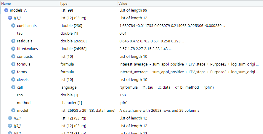
models_A <- future_map(taus, ~ rq(reg_formula, tau = .x, data = df_bank_A, method = 'pfn' ), .progress = T )

models_B <- future_map(taus, ~ rq(reg_formula, tau = .x, data = df_bank_B, method = 'pfn' ), .progress = T)

models_C <- future_map(taus, ~ rq(reg_formula, tau = .x, data = df_bank_C, method = 'pfn' ), .progress = T)

future:::ClusterRegistry("stop") # close workers. 

For each bank we get 99 quantile regressions packed in a list object.

Predictions

In research, we computed the simulation for each loan in the data. Then, we reported summary statistics about the possible savings consumers could have had if they could and knew how to ask for bids from more banks. here, a small data-set will suffice.

load('mortgage_data/data_3_for_predictions.RData')

For each bank we run the predictions separately.
The next function computes the predictions for each list of models.

# create predictions
f_predict <- function(.models , .data, .bank){
  # run pfedictions for each of the 9 models
  x1 <- map_dfc(.models, ~ predict(.x, .data)) %>% rownames_to_column(var = "id") 
  
  # arrange the data into long format to use with ggplot
  x2 <- x1 %>% gather( key = "quantile", value = "prediction", 2:ncol(x))
  x2 <- x2 %>% mutate(quantile = as.numeric(str_extract(quantile, "\\d+")),
                      bank = .bank)
  x2
}

p_bank_A <- f_predict(models_A, df_for_predictions, "A")
p_bank_B <- f_predict(models_B, df_for_predictions, "B")
p_bank_C <- f_predict(models_C, df_for_predictions, "C")

# bind  all predictions
p_banks <- bind_rows(p_bank_A, p_bank_B, p_bank_C) %>% mutate(id = as.numeric(id))

Lets see what we got:

head(p_banks %>% arrange(id))

# A tibble: 6 x 4
     id quantile prediction bank 
  <dbl>    <dbl>      <dbl> <chr>
1     1        1       2.45 A    
2     1        2       2.55 A    
3     1        3       2.57 A    
4     1        4       2.60 A    
5     1        5       2.59 A    
6     1        6       2.58 A    

For each loan we get 297 rows with each predicted price.

Lets look at the price distribution of a loan:

p_banks %>% filter(id == 10) %>%
  ggplot(aes(x = quantile, y = prediction, color = bank)) +
  geom_line()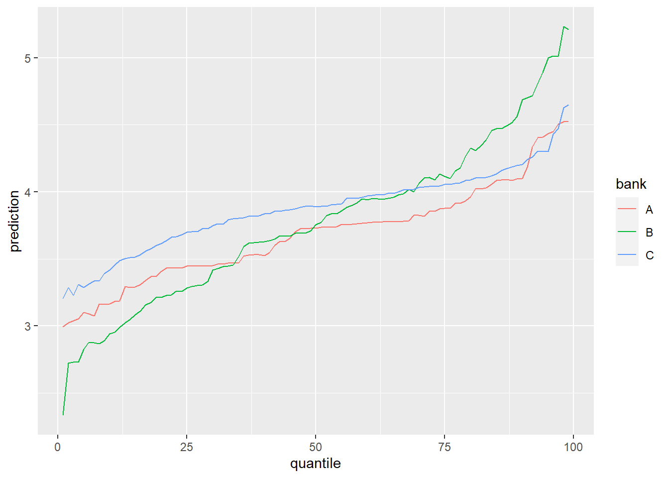

Its interesting to see that the price variance in bank B is very large. If this customer would be in the lower percentiles he is better of at bank B, but as the percentiles increase he is better of at bank A. the the end of the percentile range, the lowest price is in bank C.

Simulation

As explained above in the algorithm section, its more interesting to assume that quentiles are not determined but random. The next function draws random triplets of values \(\in [0, 99]\) for chosen quantiles and matched them to the corresponding prices. Then, for each possible combination of those price values, the minimum price is chosen. For a given loan, 7 price distributions are constructed. 3 when she goes to only one bank - for each of the 3 banks, 3 more when she bids 2 banks: AB, AC, BC, and lastly when she bids all banks.

f_simulation_dist_different_draw <- function(id_number, p_data, n = 1000) {
  # draw random quantiles for each bank
  r1 <- data.frame(
    simulation_n = rep(1:n, 3),
    id = id_number,
    bank = c(rep("A", n), rep("B", n), rep("C", n)), 
    quantile = round(runif(3 * n, 0.01, 0.99) * 100), stringsAsFactors = F )
    
 # join predictions from the p_bank Rata 
  r2 <- left_join(r1, p_data ,by = c("id", "bank", "quantile") )
  
  # For each draw triplet we choose all combinations of 2 banks,
  # As if the customer got bids from two banks.
  # There are 3 options: A-B, A-C, B-C
  r3a <- r2 %>%  select(- quantile)
  
  # option 1
  r3b1 <- r2 %>% filter(bank != "C") %>% group_by(simulation_n) %>%
    mutate(prediction = min(prediction)) %>%
    distinct(simulation_n, id, prediction) %>% ungroup() %>%
    mutate(bank = "A_B")
  
  # option 2
  r3b2 <- r2 %>% filter(bank != "B") %>% group_by(simulation_n) %>%
    mutate(prediction = min(prediction)) %>%
    distinct(simulation_n, id, prediction) %>% ungroup() %>%
    mutate(bank = "A_C")
  
  # option 3
  r3b3 <- r2 %>% filter(bank != "C") %>% group_by(simulation_n) %>%
    mutate(prediction = min(prediction)) %>%
    distinct(simulation_n, id, prediction) %>% ungroup() %>%
    mutate(bank = "B_C")
  
  
  # 1 option for bidding in all three banks
  r3c <- r2 %>% group_by(simulation_n) %>%
    mutate(prediction = min(prediction)) %>%
    distinct(simulation_n, id, prediction) %>% ungroup() %>%
    mutate(bank = "all_3_banks")
  
  # bind everything together
  r4 <- bind_rows(r3a,r3b1, r3b2, r3b3, r3c)
  
  # a Dummy variable to choose from which bank the customer is
  r4 <- r4 %>%
    mutate(A = if_else( bank %in% c("A", "A_B", "A_C", "all_3_banks"), 1, 0),
           B = if_else( bank %in% c("B", "A_B", "B_C", "all_3_banks"), 1, 0),
           C = if_else( bank %in% c("C", "A_C", "B_C", "all_3_banks"), 1, 0))
  
  r4
}

Lets simulate the price distributions for loan 10:

customer_10 <- f_simulation_dist_different_draw(id_number = 10,  p_banks)

We got a data ready to plot:

head(customer_10)

  simulation_n id bank prediction A B C
1            1 10    A       4.09 1 0 0
2            2 10    A       4.41 1 0 0
3            3 10    A       3.18 1 0 0
4            4 10    A       3.82 1 0 0
5            5 10    A       3.53 1 0 0
6            6 10    A       3.34 1 0 0

It’s not easy to look at 7 distributions simultaneously as well as in this case it doesn’t really make sense. If the customer originally was from bank C (where she runs her checking account and inclined to ask for a mortgage there), than we would like to see what she could have gained from an additional bid from bank A, B or both.

The f_plot function plots 4 distributions from the perspective of a certain bank’s customer:

f_plot <- function(data, bank_choice){
  data %>% filter(.data[[bank_choice]] == 1)  %>%
    ggplot(aes(x = prediction, color = bank, fill = bank)) +
    geom_density(alpha = 0.1) 
}

f_plot(customer_10, 'C')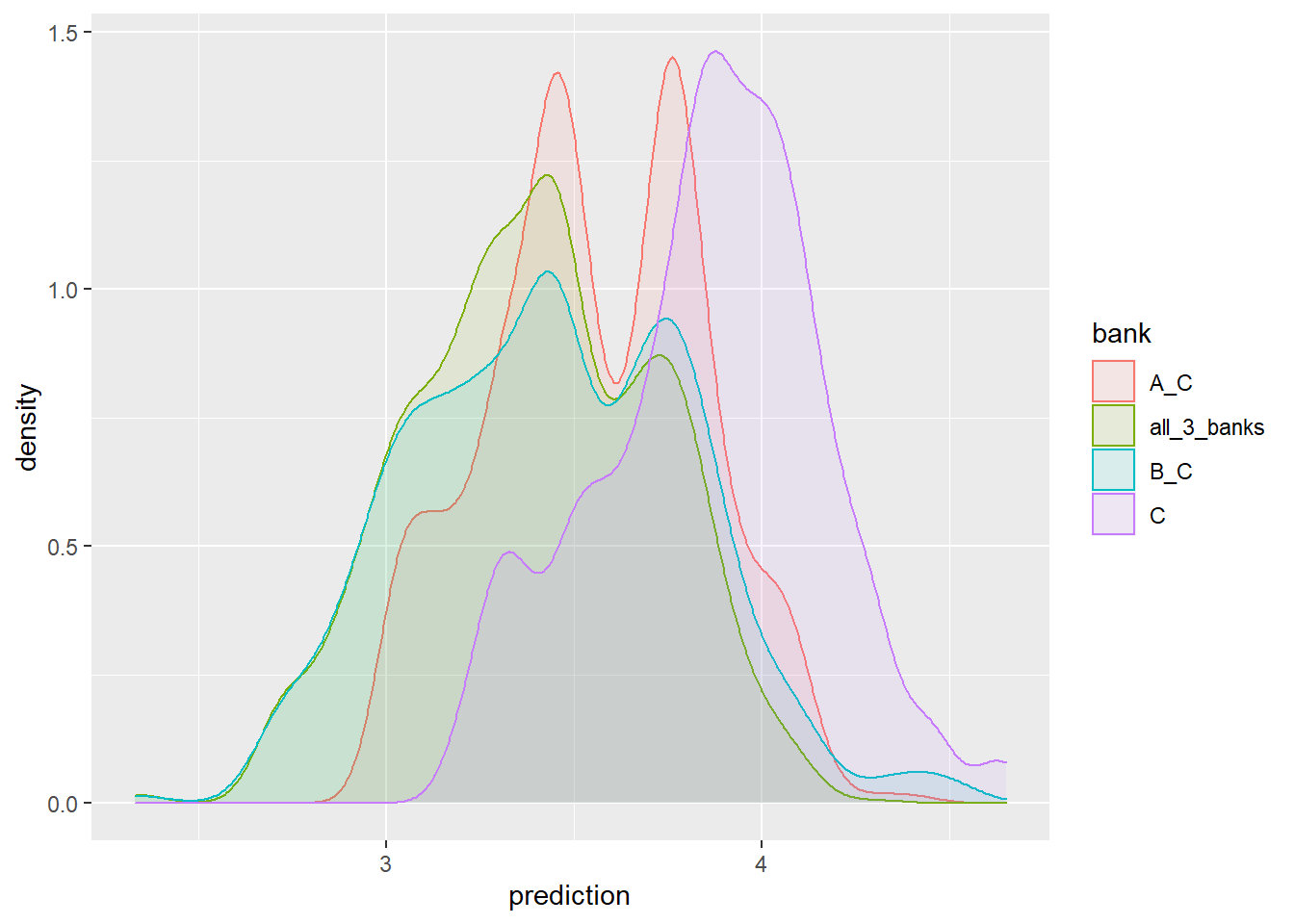

We can also look at it from every angle

p4 <- f_plot(customer_10, "A") + coord_cartesian(xlim = c(2.2, 5))
p5 <- f_plot(customer_10, "B")+ coord_cartesian(xlim = c(2.2, 5))
p6 <- f_plot(customer_10, "C")+ coord_cartesian(xlim = c(2.2, 5))

library(patchwork)
p4 / p5 / p6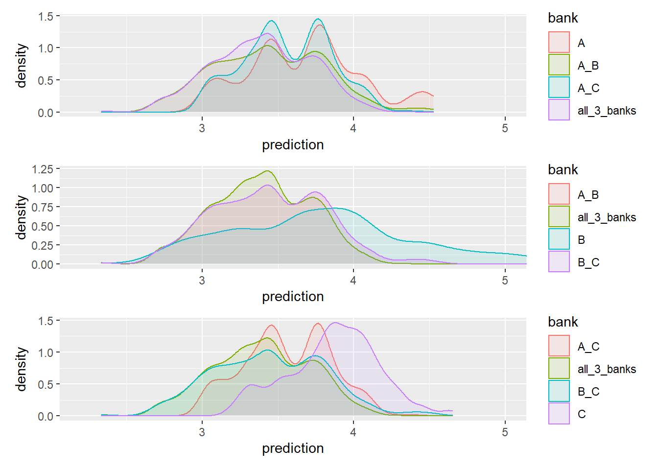

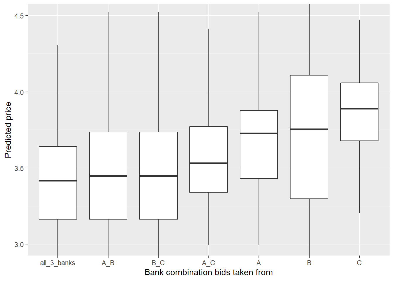
Lets take it with a boxplot:

ggplot(customer_10,
       aes(x = fct_reorder(bank, prediction, .fun = median),y = prediction)) +
  geom_boxplot() +
  coord_cartesian(ylim = c(3, 4.5)) +
  labs(x = "Bank combination bids taken from",
       y = "Predicted price")